Phylogenetic Models

Back to the Rhinograds: Phylogenetic Structural Equation Models (PhyBaSE) with `because`

One of the core features of the because package is the ability to fit Phylogenetic Bayesian Structural Equation models (PhyBaSE) through the because.phybase module, allowing researchers to account for shared evolutionary history among species when analysing the causal relationships among traits.

Once again we will use the Rhinogradentia dataset and tree previously analysed in Gonzalez-Voyer and von Hardenberg, (2014) and in von Hardenberg and Gonzalez-Voyer (2025). Let’s start by loading the necessary packages and data:

library(because.phybase) #the main `because` package will be loaded automatically 

data(rhino.dat)
data(rhino.tree)

While in previous implementations it was necessary to compute the variance-covariance matrix from the tree and pass it to JAGS, because handles this internally. You only need to provide the phylogenetic tree (class phylo) via the structure argument. Also, because automatically matches the species names in the data and tree: you only need to ensure that the species names in the data frame column specified by species match the tip labels in the tree and provide the name of the species column to the because() function through the id_col argument. Also, you do not need to rescale the total tree length to 1 (needed for a correct estimation of Pagel’s lambda parameter), as because will handle this internally.

So, let’s specify the structural equations of the best model (sem8) as fitted by von Hardenberg and Gonzalez-Voyer (2025):

sem8_eq <- list(
    LS ~ BM,
    NL ~ BM + RS,
    DD ~ NL
)

plot_dag(sem8_eq)

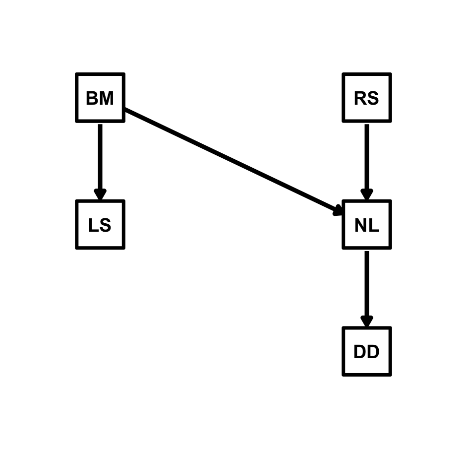
Now we can fit the model with because() including the phylogenetic tree with the structure argument. Also, as this is a more complex model than in the previous examples, to speed up the model fitting we will run 3 chains in parallel using the parallel = TRUE and n.cores = 3 arguments. Also we will request the WAIC information criterion to be computed by setting WAIC = TRUE:

fit_sem8 <- because(
    equations = sem8_eq,
    data = rhino.dat,
    structure = rhino.tree,
    id_col = "SP",
    WAIC = TRUE,
    parallel = TRUE,
    n.cores = 3
)

summary(fit_sem8)

#                  Mean    SD Naive SE Time-series SE   2.5%    50% 97.5%
# alphaDD         0.581 0.276    0.005          0.007  0.036  0.582 1.146
# alphaLS         0.344 0.416    0.008          0.016 -0.490  0.346 1.138
# alphaNL        -0.055 0.339    0.006          0.015 -0.731 -0.054 0.601
# beta_DD_NL      0.536 0.074    0.001          0.001  0.390  0.538 0.682
# beta_LS_BM      0.472 0.085    0.002          0.002  0.309  0.470 0.641
# beta_NL_BM      0.470 0.068    0.001          0.001  0.336  0.471 0.604
# beta_NL_RS      0.597 0.068    0.001          0.001  0.461  0.596 0.728
# lambdaDD        0.462 0.130    0.002          0.003  0.218  0.462 0.717
# lambdaLS        0.696 0.107    0.002          0.003  0.459  0.709 0.862
# lambdaNL        0.719 0.086    0.002          0.002  0.533  0.727 0.863
# sigma_DD_phylo  0.803 0.174    0.003          0.003  0.503  0.790 1.178
# sigma_DD_res    0.856 0.088    0.002          0.002  0.694  0.852 1.041
# sigma_LS_phylo  1.253 0.204    0.004          0.005  0.865  1.246 1.675
# sigma_LS_res    0.804 0.104    0.002          0.002  0.615  0.802 1.013
# sigma_NL_phylo  1.026 0.145    0.003          0.004  0.766  1.013 1.338
# sigma_NL_res    0.626 0.075    0.001          0.002  0.490  0.622 0.783
#                 Rhat n.eff
# alphaDD        1.000  1408
# alphaLS        1.003   639
# alphaNL        1.000   553
# beta_DD_NL     1.000  3088
# beta_LS_BM     1.001  2178
# beta_NL_BM     1.000  2255
# beta_NL_RS     1.001  2801
# lambdaDD       1.002  2136
# lambdaLS       1.000  1595
# lambdaNL       1.001  1788
# sigma_DD_phylo 1.002  2741
# sigma_DD_res   1.000  2712
# sigma_LS_phylo 1.000  1612
# sigma_LS_res   1.001  2103
# sigma_NL_phylo 1.001  1600
# sigma_NL_res   1.001  2427
# 
# DIC:
# Mean deviance:  670 
# penalty 133.7 
# Penalized deviance: 803.6 
# 
# WAIC:
# WAIC with Standard Errors
# -------------------------
# N = 300 observations, 3000 MCMC samples
# 
#           Estimate   SE
# elpd_waic   -395.1  9.9
# p_waic        93.7  5.1
# waic         790.2 19.8

The output shows that the posterior parameters are consistent with those we obtained coding the model directly in JAGS (von Hardenberg and Gonzalez-Voyer, 2025; the code is available in the supplementary materials of the paper).

The random effects formulation of because

If you are familiar with the output obtained from that model, you may however have noticed that besides Pagel’s $\lambda$ parameters for each response variable, with because() we also get estimates of the standard deviations of the phylogenetic and residual components (sigma_[RESP]_phylo and sigma_[RESP]_res, respectively). These are estimated because because uses an optimised random effect formulation to improve MCMC and significantly reduce runtime. While standard phylogenetic models must invert the covariance matrix at every iteration (as $\lambda$ changes), the random effect approach is mathematically equivalent but computationally more efficent. because decomposes the response into three additive components:

$y_i = \mu_i + u_i + \epsilon_i$

where:

$\mu_i$ is the fixed effect (structural equation mean)
$u_i$ is the phylogenetic random effect: $\mathbf{u} \sim \mathcal{N}(\mathbf{0}, \sigma_u^2 \mathbf{V})$
$\epsilon_i$ is the residual error: $\boldsymbol{\epsilon} \sim \mathcal{N}(\mathbf{0}, \sigma_e^2 \mathbf{I})$

This allows us to pre-compute the inverse phylogenetic variance-covariance matrix ( $\mathbf{V}^{-1}$ ) only once and pass it to JAGS as fixed data. JAGS simply scales this fixed precision matrix by 1/ $\sigma$ , avoiding costly repeated inversions.

Consequently, $\lambda$ is derived from the posterior variance components as: $\lambda = \frac{\sigma_{phylo}^2}{\sigma_{phylo}^2 + \sigma_{res}^2}$

This is the approach also used in other packages such as MCMCglmm (Hadfield, 2010) and brms (Bürkner, 2017).

Improved WAIC calculation

In because we improved the WAIC calculation, compared to how we calculated it in von Hardenberg & Gonzalez-Voyer, (2025). The WAIC is now computed directly from the pointwise log-likelihoods monitored during model fitting, rather than approximating it from the deviance as done previously. This approach, besides providing more accurate estimates of the WAIC than the deviance-based approximation provided by JAGS, also allows us to compute the standard errors for WAIC (following the method suggested by Vehtari et al. 2017) allowing for more reliable model comparisons.

Testing conditional independencies with d-separation

Let’s now test the conditional independencies implied by the model (We will set WAIC = FALSE here to speed up the computation, as we do not need to compare models):

test_sem8_dsep <- because(
    equations = sem8_eq,
    data = rhino.dat,
    structure = rhino.tree,
    id_col = "SP",
    dsep = TRUE,
    WAIC = FALSE,
    parallel = TRUE,
    n.cores = 3
)

summary(test_sem8_dsep)

# d-separation Tests
# ==================
# 
# Test: RS _||_ BM | {}  
#   Parameter Estimate LowerCI UpperCI Indep    P  Rhat n.eff
#  beta_RS_BM   -0.029  -0.238   0.177   Yes 0.78 1.002  2177
# 
# Test: RS _||_ DD | {NL} 
#   Parameter Estimate LowerCI UpperCI Indep     P Rhat n.eff
#  beta_RS_DD   -0.117   -0.33   0.107   Yes 0.301    1  2563
# 
# Test: RS _||_ LS | {BM} 
#   Parameter Estimate LowerCI UpperCI Indep     P Rhat n.eff
#  beta_RS_LS   -0.019  -0.248    0.22   Yes 0.873    1  2423
# 
# Test: BM _||_ DD | {NL} 
#   Parameter Estimate LowerCI UpperCI Indep     P Rhat n.eff
#  beta_BM_DD    0.117  -0.111   0.342   Yes 0.322    1  1824
# 
# Test: NL _||_ LS | {RS,BM} 
#   Parameter Estimate LowerCI UpperCI Indep    P Rhat n.eff
#  beta_NL_LS    0.013  -0.151   0.177   Yes 0.86    1  2134
# 
# Test: DD _||_ LS | {NL,BM} 
#   Parameter Estimate LowerCI UpperCI Indep     P  Rhat n.eff
#  beta_DD_LS   -0.063  -0.245   0.114   Yes 0.495 1.002  2693
# 
# 
# Legend:
#   Indep: 'Yes' = Conditionally Independent, 'No' = Dependent (based on 95% CI)
#   P: Bayesian probability that the posterior distribution overlaps with zero

As expected, all conditional independencies are supported, indicating that the the hypothesised causal structure is consistent with the data.

Accounting for measurement error in traits in PhyBaSE models

In von Hardenberg and Gonzalez-Voyer (2025), we showed how PhyBaSE models can be specified to account for measurement error in the traits. These models can also be fitted with because(). In the case you have available repeated measures per species, it is sufficient to provide the data frame with all measurements (i.e. multiple rows per species) and specify the id_col argument to indicate the species identifier column. because() will automatically format the data to create a response matrix with species in rows and replicates in columns, padding with NAs as necessary. We will use the same data simulated in von Hardenberg and Gonzalez-Voyer (2025) for this example. Each trait was transformed to a distribution with mean equal to the original species trait value in rhino.dat and SD equal to a proportion (25%) of the among-species variance for that trait. Then 10 repeated measures were sampled for each species. The resulting data frame RhinoMulti.dat contains 1000 rows (10 replicates for each of the 100 species) and 6 columns (species identifier and 5 traits). Let’s load the data and fit the same model as before accounting for the repeated measures:

library(because)
data(RhinoMulti.dat)
data(rhino.tree)

RhinoMulti.eq <-list(
    LS ~ BM,
    NL ~ BM + RS,
    DD ~ NL
  )

RhinoMulti.bc <- because(
  equations = RhinoMulti.eq,
  data = RhinoMulti.dat,
  structure = rhino.tree,
  id_col = "SP", # species identifier column
  variability = "reps", # specify that data contains repeated measures
  parallel = TRUE,
  n.cores = 3
)


summary(RhinoMulti.bc)

#                  Mean    SD Naive SE Time-series SE   2.5%    50%
# alphaDD         0.593 0.291    0.005          0.008  0.043  0.588
# alphaLS         0.381 0.394    0.007          0.016 -0.384  0.384
# alphaNL        -0.084 0.321    0.006          0.012 -0.722 -0.085
# beta_DD_NL      0.539 0.079    0.001          0.001  0.383  0.539
# beta_LS_BM      0.446 0.084    0.002          0.002  0.287  0.445
# beta_NL_BM      0.466 0.068    0.001          0.001  0.333  0.465
# beta_NL_RS      0.592 0.069    0.001          0.001  0.463  0.592
# lambdaDD        0.484 0.134    0.002          0.003  0.221  0.485
# lambdaLS        0.698 0.106    0.002          0.003  0.453  0.708
# lambdaNL        0.696 0.091    0.002          0.002  0.503  0.705
# sigma_DD_phylo  0.826 0.178    0.003          0.004  0.516  0.813
# sigma_DD_res    0.842 0.094    0.002          0.002  0.668  0.839
# sigma_LS_phylo  1.249 0.206    0.004          0.005  0.869  1.234
# sigma_LS_res    0.796 0.105    0.002          0.002  0.607  0.790
# sigma_NL_phylo  0.997 0.146    0.003          0.004  0.739  0.986
# sigma_NL_res    0.644 0.079    0.001          0.002  0.501  0.641
#.                97.5%  Rhat n.eff
# alphaDD        1.171 1.000  1295
# alphaLS        1.140 1.000   655
# alphaNL        0.545 1.001   744
# beta_DD_NL     0.693 1.000  2902
# beta_LS_BM     0.609 1.000  2205
# beta_NL_BM     0.602 1.001  2320
# beta_NL_RS     0.729 1.001  2916
# lambdaDD       0.735 1.000  1970
# lambdaLS       0.872 1.000  1448
# lambdaNL       0.853 1.000  1653
# sigma_DD_phylo 1.210 1.000  2057
# sigma_DD_res   1.039 1.000  2370
# sigma_LS_phylo 1.682 1.000  1445
# sigma_LS_res   1.021 1.000  1907
# sigma_NL_phylo 1.307 1.001  1503
# sigma_NL_res   0.816 1.000  2363

In von Hardenberg and Gonzalez-Voyer (2025) we showed also how to account for measurement error when only a single observation per species is available, but the measurement standard error is known. This can also be done with because() by providing for each trait a second collumn called [TRAIT]_se containing the standard error of the measurements for each species.

library(because)
data(RhinoMulti_se.dat)
data(rhino.tree)

RhinoMulti_se.bc <- because(
  equations = RhinoMulti.eq,
  data = RhinoMulti_se.dat,
  structure = rhino.tree,
  id_col = "SP",
  variability = "se", # specify that data contains standard errors
  parallel = TRUE,
  n.cores = 3
)

summary(RhinoMulti_se.bc)

#                  Mean    SD Naive SE Time-series SE   2.5%    50% 97.5%  Rhat
# alphaDD         0.581 0.289    0.005          0.008  0.003  0.577 1.132 1.002
# alphaLS         0.372 0.412    0.008          0.016 -0.435  0.373 1.188 1.003
# alphaNL        -0.117 0.352    0.006          0.015 -0.821 -0.125 0.587 1.002
# beta_DD_NL      0.541 0.077    0.001          0.001  0.392  0.541 0.691 1.000
# beta_LS_BM      0.442 0.086    0.002          0.002  0.275  0.441 0.612 1.000
# beta_NL_BM      0.466 0.069    0.001          0.002  0.331  0.465 0.603 1.000
# beta_NL_RS      0.591 0.069    0.001          0.002  0.450  0.591 0.721 1.000
# lambdaDD        0.492 0.135    0.002          0.003  0.238  0.494 0.751 1.001
# lambdaLS        0.700 0.105    0.002          0.003  0.463  0.713 0.866 1.006
# lambdaNL        0.701 0.090    0.002          0.002  0.505  0.709 0.854 1.000
# sigma_DD_phylo  0.833 0.181    0.003          0.004  0.515  0.823 1.224 1.000
# sigma_DD_res    0.832 0.091    0.002          0.002  0.663  0.828 1.017 1.000
# sigma_LS_phylo  1.252 0.201    0.004          0.005  0.872  1.240 1.666 1.010
# sigma_LS_res    0.796 0.106    0.002          0.002  0.602  0.790 1.020 1.002
# sigma_NL_phylo  1.005 0.148    0.003          0.004  0.743  0.996 1.326 1.000
# sigma_NL_res    0.642 0.078    0.001          0.002  0.500  0.640 0.808 1.000
#                n.eff
# alphaDD         1237
# alphaLS          647
# alphaNL          579
# beta_DD_NL      2969
# beta_LS_BM      1712
# beta_NL_BM      2036
# beta_NL_RS      2055
# lambdaDD        2086
# lambdaLS        1571
# lambdaNL        1454
# sigma_DD_phylo  2147
# sigma_DD_res    2561
# sigma_LS_phylo  1553
# sigma_LS_res    2205
# sigma_NL_phylo  1501
# sigma_NL_res    2184

Accounting for uncertainity in the phylogenetic tree

In cases where there is uncertainty about the phylogenetic relationships among species, because allows users to fit models across a sample of trees as described in von Hardenberg and Gonzalez Voyer, 2025). With because this becomes trivial: You just need to provide a list of phylogenetic trees (class multiPhylo) to the structure argument instead of a single tree; because will then randomly sample one tree from the list at each MCMC iteration, effectively integrating over phylogenetic uncertainty when estimating model parameters.

References

von Hardenberg, A. and Gonzalez-Voyer, A. (2025). PhyBaSE: A Bayesian approach to Phylogenetic Structural Equation Models. Methods in Ecology and Evolution. https://doi.org/10.1111/2041-210X.70044

Vehtari, A., Gelman, A., & Gabry, J. (2017). Practical Bayesian model evaluation using leave-one-out cross-validation and WAIC. Statistics and Computing, 27(5), 1413-1432.

Achaz von Hardenberg

2026-04-16

Back to the Rhinograds: Phylogenetic Structural Equation Models (PhyBaSE) with `because`

The random effects formulation of because

Improved WAIC calculation

Testing conditional independencies with d-separation

Accounting for measurement error in traits in PhyBaSE models

Accounting for uncertainity in the phylogenetic tree

References

Phylogenetic Models

Achaz von Hardenberg

2026-04-16

Back to the Rhinograds: Phylogenetic Structural Equation Models (PhyBaSE) with because

The random effects formulation of because

Improved WAIC calculation

Testing conditional independencies with d-separation

Accounting for measurement error in traits in PhyBaSE models

Accounting for uncertainity in the phylogenetic tree

References

Back to the Rhinograds: Phylogenetic Structural Equation Models (PhyBaSE) with `because`